|
|
Your source of photonics CAD tools | |
|
| ||
FIMMWAVEA powerful waveguide mode solver |
    |
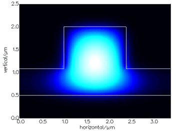
The FMM SolverThe FMM Solver, a fully vectorial solver based on the Film Mode Matching Method, is the perfect solver for waveguide structures with a rectangular geometry. It is a semi-analytic method that does not need any discretisation of the structure, provided the structure can be well described by a finite set of rectangles. This makes it very efficient to model waveguides that have very small features or are very wide, or both. It is ideal for epitaxially grown structures that might include very thin layers such as quantum wells.
Features:Fully-vectorial and semi-vectorial versions The FMM Solver supports perfect electric wall and perfect magnetic wall boundary conditions, Impedance boundary conditions (anywhere between the perfect electric wall and the perfect magnetic wall), Transparent boundary conditions, periodic boundary conditions and Perfectly Matching Layers (PMLs).. Structures for which the FMM Solver is recommended:Waveguides with a rectangular geometry, or a geometry that can be simply discretised into rectangles See also the Mode Solver Features Table for comparison with other solvers. The method:The Mode Matching Method models an arbitrary waveguide by a list of vertical slices, each uniform laterally, but composed vertically of a number of layers. A 2D mode is built up from the TE and TM 1D modes of each slice. The method is theoretically exact for an infinite number of 1D modes. The modelled area may be bound by either perfect metallic or magnetic walls or with periodic boundary conditions. The FMM Solver support PMLs, impedance or transparent boundary conditions. The method will happily deal with modes that are near cut-off in the lateral direction, without loss of accuracy or an increase in computation time. Such modes cannot be modelled accurately with finite element or finite difference methods. Speed:Locating the zero order mode of a 4-slice ridge structure with a resolution of 30 2D modes will take about 2s on a 2GHz Pentium IV using the Molab (see below). If you had some idea of where it is, it might take 1s and regenerating it from an accurate eigenvalue will take a fraction of a second. The calculation time is proportional to the number of slices in your structure; it barely increases at all with an increased number of layers (vertical structure resolution).
|
 © 2023 Photon Design copyright all rights reserved |

 |