|
|
Your source of photonics CAD tools | |
|
| ||
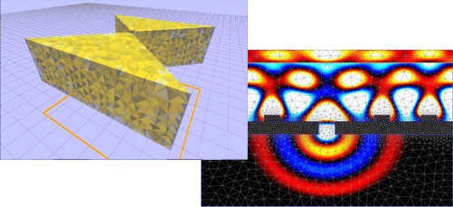
OmniSim FETDOmni-directional photonics FETD simulations |
    |
FETD Simulation Software with OmniSimPart of our state-of-the-art FDTD and FETD time-domain toolkitFinite element time domain (FETD) simulations are an alternative to the popular finite difference time domain (FDTD) method. Incorporating innovative proprietary techniques, Photon Design presents an efficient, fully-functional FETD calculation engine, which complements our state-of-the-art FDTD engine for simulations of photonic devices. The FETD engine is designed to address some of the specific shortcomings of FDTD, in particular when modelling plasmonics and metamaterials: FDTD can be very slow when dealing with metallic structures and plasmonic devices. In these areas, the FETD engine delivers major steps forward in terms of capability and efficiency. Our FETD engine is also much faster than finite element frequency domain (FEFD) methods for all but the smallest structures. FETD is also ideal for modelling graphene-based devices or other 2D materials; it can deal with such structures extremely efficiently using a native surface material model. With this new addition to OmniSim and CrystalWave, Photon Design offers the world’s first integrated FDTD and FETD simulation suite. You can now choose the most efficient calculation method for your structure, and you can also model your design with two independent engines - ideal to check the accuracy of your simulations!
Features
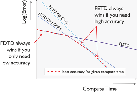
Why combine FDTD and FETD?A combination of FDTD and FETD offers you the best of both worlds: FDTD for fast initial calculations, and FETD when high accuracy is needed. FDTD is a very fast method for obtaining results with a modest accuracy in a small amount of time, however as a method it scales poorly with resolution, bringing little gain in accuracy as computation time increases. FETD uses higher order elements than FDTD and as a result it converges much faster, so it will allow you to obtain highly accurate results more quickly. This is summarised in the diagram below.
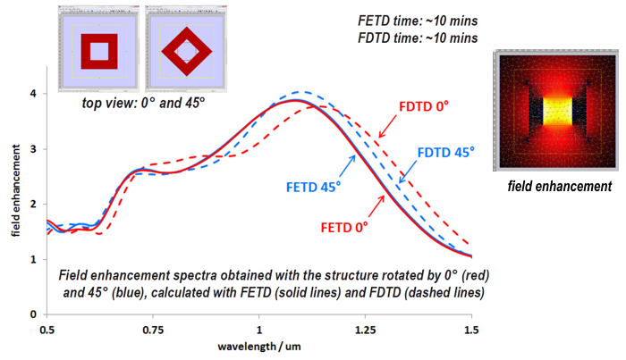
Body-conformal meshingThanks to its adaptive mesh, the FETD engine is much less orientation-sensitive than FDTD. This allows it to deal with slanted or curved interfaces with no staircase approximation and no material averaging at the surface. We simulated a gold nut structure with two different orientations and calculated the field enhancement in the centre of the hole. The FDTD engine displays erroneous discrepancies between the two orientations, caused by the staircase approximation of the diagonal interface at that resolution. For the same calculation time, the FETD engine gives almost identical results for both orientations for the entire spectrum.
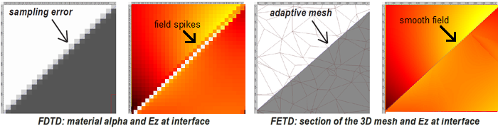
You can see below some of the effects of the staircasing in the rotated structure. The FDTD grid and field are shown on the left-hand side; note the spikes! On the right-hand side you can see a section of the adaptive FETD mesh and the corresponding field, without unwanted spikes this time.
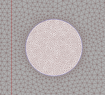
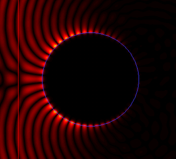
This is ideal when modelling curved interfaces, particularly for metals. You can see below the 2D triangular adaptive mesh around a gold cylinder. Note how the mesh conforms to the edges of the cylinder and how the triangles get smaller close to the metal, where higher resolution is needed for the fields (plotted on the right).
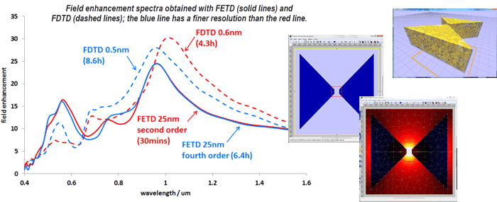
Superior convergenceModelling an inclined metal surface in 3D can be a major challenge for FDTD, as extremely small grids are required to obtain accurate results. In this example we measured electric field enhancement in the hole of a bow-tie antenna. The FDTD simulation still had not converged after an 8h30 simulation on a i7-860 CPU (4 cores) and was unable to locate the resonant wavelength and the amplitude of the resonant peak with precision. On the same computer the FETD algorithm converged with a calculation time of only 30 minutes! Such efficiency is made possible by the use of higher order elements in the finite-element mesh and by the FETD’s ability to avoid staircasing at the metal surface.
Bloch boundary conditionsThe FETD engine supports true Bloch boundary conditions to simulate 1D-periodic and 2D-periodic structures with oblique illumination using a single unit cell. Structures with periodicity in 1 dimension are performed with the 2D FETD engine and structures with 2D periodicity are performed with the 3D FETD engine This will allow you to simulate the propagation of light incident on 1D- or 2D-periodic structures such as
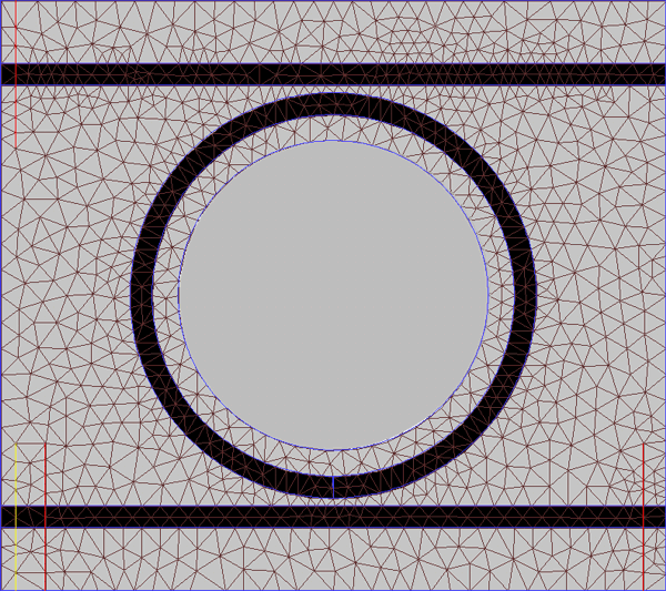
The illumination can be set with one degree of freedom for 1D-periodic gratings (angle in plane of the grating) and two degrees of freedom for 2D-periodic gratings. The Bloch boundary condition has broadband capability and can thus be used to obtain the spectrum of a an obliquely-illuminated periodic structure in a single time-domain simulation. The Bloch boundary condition imposes no additional memory requirement and only a small overhead in terms of computation time compared with standard FETD. Mesh voidsWith the FETD engine you can speed up calculations by defining "void regions": empty regions where no computation is needed. This can be applied to regions where light does not penetrate, or regions where light would be assumed to be lost, for instance inside a ring resonator or in the centre of a large metallic volume. You can see an example below with a ring resonator: note the region without mesh inside the ring.
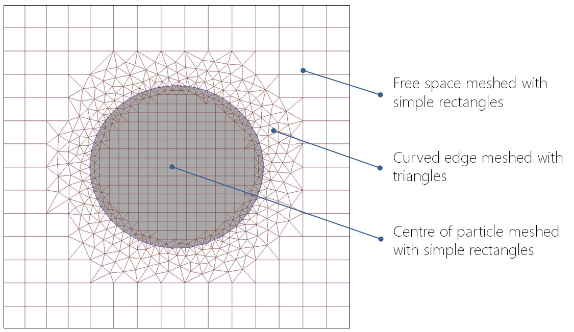
Hybrid meshWith the FETD hybrid meshing, the calculator will use both rectangular and triangular elements in 2D (or cuboid and tetrahedral in 3D) to substantially reduce the runtime of the simulation. The triangular elements conform closely to the boundaries of more complex regions (such as tilted sides or curves), while the less computationally demanding rectangular elements will model open spaces. The rectangles (cuboids) are also much more efficient at meshing thin layers than triangles (tetrahedra).
Download OmniSim for nanophotonics brochure
|
 © 2023 Photon Design copyright all rights reserved |

 |